Human Activity Recognition from Smartphone Sensors#
PCA, KMeans Clustering and Supervised Classification#
Goal#
This notebook studies whether smartphone sensor features reveal human activities in two ways:
Unsupervised exploration: PCA and KMeans discover activity-like groups without using the activity labels while building clusters.
Supervised prediction: Logistic Regression, Random Forest and XGBoost predict activity labels for volunteers in the official unseen test set.
The dataset contains motion windows from 30 volunteers performing six activities. Each row contains 561 prepared sensor features. The official train/test split is preserved: model tuning happens only with the training volunteers, and the test set is checked only at the final stage.
Source: UCI Human Activity Recognition Using Smartphones
# Run only if needed:
# !pip install umap-learn xgboost -q
1. Load the data#
from pathlib import Path
import pandas as pd

train = pd.read_csv("../data/sensor_train.csv")
test = pd.read_csv("../data/sensor_test.csv")

feature_columns = [c for c in train.columns if c not in ["subject", "Activity"]]

summary = pd.DataFrame({
    "Set": ["Train", "Test"],
    "Rows": [len(train), len(test)],
    "Sensor features": [len(feature_columns), len(feature_columns)],
    "Volunteers": [train["subject"].nunique(), test["subject"].nunique()],
    "Activities": [train["Activity"].nunique(), test["Activity"].nunique()],
    "Missing values": [train.isna().sum().sum(), test.isna().sum().sum()]
})

summary
| Set | Rows | Sensor features | Volunteers | Activities | Missing values | |
|---|---|---|---|---|---|---|
| 0 | Train | 7352 | 561 | 21 | 6 | 0 |
| 1 | Test | 2947 | 561 | 9 | 6 | 0 |
train["Activity"].value_counts().rename_axis("Activity").to_frame("Train rows")
| Train rows | |
|---|---|
| Activity | |
| LAYING | 1407 |
| STANDING | 1374 |
| SITTING | 1286 |
| WALKING | 1226 |
| WALKING_UPSTAIRS | 1073 |
| WALKING_DOWNSTAIRS | 986 |
X_train = train[feature_columns]
y_train = train["Activity"]
groups_train = train["subject"]

X_test = test[feature_columns]
y_test = test["Activity"]

X_train.shape, X_test.shape
((7352, 561), (2947, 561))
The Activity label is used only after clustering for evaluation, and later as the target for classification. The subject column identifies volunteers and is used to make cross-validation group-aware.
2. PCA dimensionality reduction#
import numpy as np
from sklearn.decomposition import PCA

pca_full = PCA(random_state=42)
pca_full.fit(X_train)

cumulative_variance = np.cumsum(pca_full.explained_variance_ratio_)

pca_report = pd.DataFrame({
    "PCA components": [2, 5, 10, 11, 36, 50, 69],
    "Variance retained (%)": [
        cumulative_variance[1] * 100,
        cumulative_variance[4] * 100,
        cumulative_variance[9] * 100,
        cumulative_variance[10] * 100,
        cumulative_variance[35] * 100,
        cumulative_variance[49] * 100,
        cumulative_variance[68] * 100
    ]
}).round(2)

pca_report
| PCA components | Variance retained (%) | |
|---|---|---|
| 0 | 2 | 67.47 |
| 1 | 5 | 75.16 |
| 2 | 10 | 80.50 |
| 3 | 11 | 81.27 |
| 4 | 36 | 90.55 |
| 5 | 50 | 93.09 |
| 6 | 69 | 95.23 |
import matplotlib.pyplot as plt

fig, ax = plt.subplots(figsize=(9, 5))
ax.plot(range(1, 81), cumulative_variance[:80] * 100, marker="o", markersize=3)
ax.axhline(90, linestyle="--", linewidth=1, label="90%")
ax.axhline(95, linestyle="--", linewidth=1, label="95%")
ax.axvline(50, linestyle=":", linewidth=1, label="50 PCs")
ax.axvline(69, linestyle=":", linewidth=1, label="69 PCs")
ax.set_title("PCA Cumulative Explained Variance")
ax.set_xlabel("Number of PCA components")
ax.set_ylabel("Variance retained (%)")
ax.legend()
ax.grid(False)
plt.tight_layout()
plt.show()
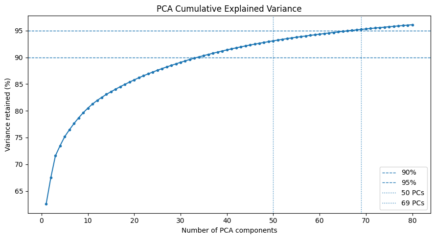
We report PCA with 36, 50 and 69 components for clustering. For the supervised models, we use only PCA 69, because it preserves approximately 95% of training variation while still reducing the original 561 features heavily.
3. KMeans clustering after PCA#
from sklearn.cluster import KMeans
from sklearn.metrics import silhouette_score, adjusted_rand_score, normalized_mutual_info_score

clustering_results = []
cluster_labels = {}
pca_spaces = {}

for n_components in [36, 50, 69]:
    pca = PCA(n_components=n_components, random_state=42)
    X_pca = pca.fit_transform(X_train)

    kmeans = KMeans(n_clusters=6, n_init=20, random_state=42)
    clusters = kmeans.fit_predict(X_pca)

    clustering_results.append({
        "PCA components": n_components,
        "Variance retained (%)": pca.explained_variance_ratio_.sum() * 100,
        "Silhouette": silhouette_score(X_pca, clusters, sample_size=3000, random_state=42),
        "ARI": adjusted_rand_score(y_train, clusters),
        "NMI": normalized_mutual_info_score(y_train, clusters)
    })

    cluster_labels[n_components] = clusters
    pca_spaces[n_components] = X_pca

clustering_results = pd.DataFrame(clustering_results).round(3)
clustering_results
| PCA components | Variance retained (%) | Silhouette | ARI | NMI | |
|---|---|---|---|---|---|
| 0 | 36 | 90.548 | 0.182 | 0.455 | 0.584 |
| 1 | 50 | 93.086 | 0.170 | 0.456 | 0.585 |
| 2 | 69 | 95.226 | 0.160 | 0.455 | 0.584 |
best_pca_for_clustering = int(
    clustering_results.sort_values("Silhouette", ascending=False).iloc[0]["PCA components"]
)

X_cluster_pca = pca_spaces[best_pca_for_clustering]
best_clusters = cluster_labels[best_pca_for_clustering]

best_pca_for_clustering
36
cluster_activity = pd.crosstab(
    pd.Series(best_clusters, name="KMeans cluster"),
    y_train.reset_index(drop=True).rename("Known activity"),
    normalize="index"
).mul(100).round(1)

cluster_activity
| Known activity | LAYING | SITTING | STANDING | WALKING | WALKING_DOWNSTAIRS | WALKING_UPSTAIRS |
|---|---|---|---|---|---|---|
| KMeans cluster | ||||||
| 0 | 0.7 | 0.1 | 0.0 | 37.6 | 8.7 | 53.0 |
| 1 | 0.0 | 49.2 | 50.8 | 0.0 | 0.0 | 0.0 |
| 2 | 0.0 | 0.0 | 0.0 | 40.1 | 44.5 | 15.4 |
| 3 | 16.8 | 35.5 | 47.6 | 0.0 | 0.0 | 0.0 |
| 4 | 96.1 | 3.9 | 0.0 | 0.0 | 0.0 | 0.0 |
| 5 | 0.0 | 0.0 | 0.0 | 23.8 | 64.3 | 11.9 |
fig, ax = plt.subplots(figsize=(10, 5))
image = ax.imshow(cluster_activity.values, aspect="auto")
ax.set_title(f"Cluster Composition by Known Activity — PCA {best_pca_for_clustering}")
ax.set_xlabel("Known activity")
ax.set_ylabel("KMeans cluster")
ax.set_xticks(range(len(cluster_activity.columns)))
ax.set_xticklabels(cluster_activity.columns, rotation=45, ha="right")
ax.set_yticks(range(len(cluster_activity.index)))
ax.set_yticklabels(cluster_activity.index)
ax.grid(False)
plt.colorbar(image, ax=ax, label="Percentage within cluster")
plt.tight_layout()
plt.show()
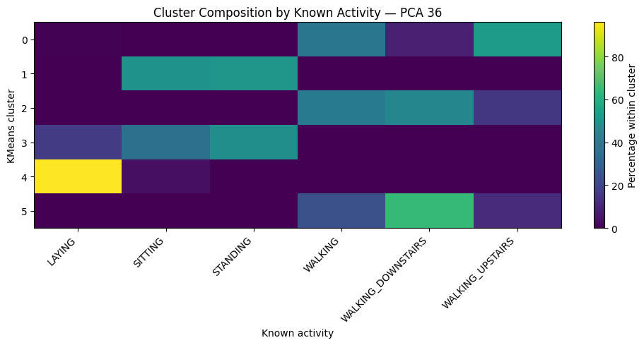
Silhouette measures natural cluster separation without using activity labels. ARI and NMI check afterward how closely the discovered clusters align with the real six activities.
4. PCA, t-SNE and UMAP visualisation#
def plot_embedding(embedding, labels, title, x_label, y_label, legend_title):
fig, ax = plt.subplots(figsize=(10, 7))
for label in sorted(pd.Series(labels).unique()):
mask = pd.Series(labels).to_numpy() == label
ax.scatter(embedding[mask, 0], embedding[mask, 1], s=18, alpha=0.78, label=label)
ax.set_title(title)
ax.set_xlabel(x_label)
ax.set_ylabel(y_label)
ax.grid(False)
ax.legend(title=legend_title, bbox_to_anchor=(1.02, 1), loc="upper left", fontsize=8)
plt.tight_layout()
plt.show()
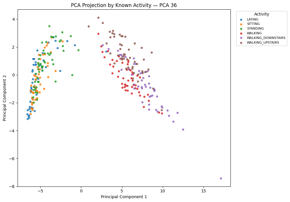
visual_sample = (
train.groupby("Activity", group_keys=False)
.sample(n=50, random_state=42)
.sample(frac=1, random_state=42)
)
visual_index = visual_sample.index
visual_activities = visual_sample["Activity"]
X_visual = X_cluster_pca[visual_index]
visual_clusters = best_clusters[visual_index]
plot_embedding(
X_visual[:, :2],
visual_activities,
f"PCA Projection by Known Activity — PCA {best_pca_for_clustering}",
"Principal Component 1",
"Principal Component 2",
"Activity"
)
from sklearn.manifold import TSNE
tsne = TSNE(
n_components=2,
perplexity=30,
init="pca",
learning_rate="auto",
max_iter=500,
random_state=42
)
X_tsne = tsne.fit_transform(X_visual)
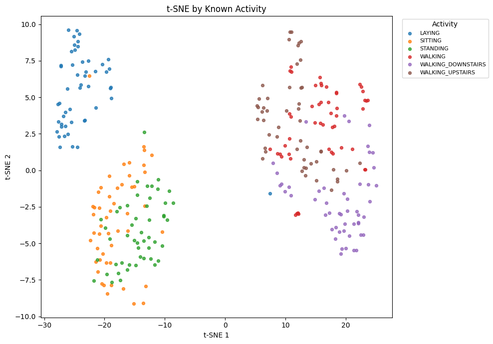
plot_embedding(X_tsne, visual_activities, "t-SNE by Known Activity", "t-SNE 1", "t-SNE 2", "Activity")
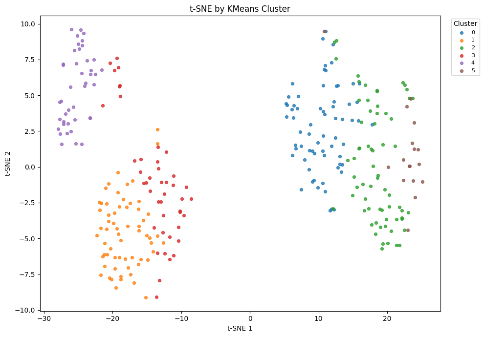
plot_embedding(X_tsne, visual_clusters, "t-SNE by KMeans Cluster", "t-SNE 1", "t-SNE 2", "Cluster")
!pip install umap-learn
Requirement already satisfied: umap-learn in C:\Users\zirad\AppData\Local\Programs\Python\Python312\Lib\site-packages (0.5.12)
Requirement already satisfied: numpy>=1.23 in C:\Users\zirad\AppData\Local\Programs\Python\Python312\Lib\site-packages (from umap-learn) (2.0.2)
Requirement already satisfied: scipy>=1.3.1 in C:\Users\zirad\AppData\Local\Programs\Python\Python312\Lib\site-packages (from umap-learn) (1.16.1)
Requirement already satisfied: scikit-learn>=1.6 in C:\Users\zirad\AppData\Local\Programs\Python\Python312\Lib\site-packages (from umap-learn) (1.7.1)
Requirement already satisfied: numba>=0.51.2 in C:\Users\zirad\AppData\Local\Programs\Python\Python312\Lib\site-packages (from umap-learn) (0.60.0)
Requirement already satisfied: pynndescent>=0.5 in C:\Users\zirad\AppData\Local\Programs\Python\Python312\Lib\site-packages (from umap-learn) (0.6.0)
Requirement already satisfied: tqdm in C:\Users\zirad\AppData\Local\Programs\Python\Python312\Lib\site-packages (from umap-learn) (4.66.1)
Requirement already satisfied: llvmlite<0.44,>=0.43.0dev0 in C:\Users\zirad\AppData\Local\Programs\Python\Python312\Lib\site-packages (from numba>=0.51.2->umap-learn) (0.43.0)
Requirement already satisfied: joblib>=0.11 in C:\Users\zirad\AppData\Local\Programs\Python\Python312\Lib\site-packages (from pynndescent>=0.5->umap-learn) (1.5.1)
Requirement already satisfied: threadpoolctl>=3.1.0 in C:\Users\zirad\AppData\Local\Programs\Python\Python312\Lib\site-packages (from scikit-learn>=1.6->umap-learn) (3.6.0)
Requirement already satisfied: colorama in C:\Users\zirad\AppData\Local\Programs\Python\Python312\Lib\site-packages (from tqdm->umap-learn) (0.4.6)
WARNING: Ignoring invalid distribution ~tatsmodels (C:\Users\zirad\AppData\Local\Programs\Python\Python312\Lib\site-packages)
WARNING: Ignoring invalid distribution ~tatsmodels (C:\Users\zirad\AppData\Local\Programs\Python\Python312\Lib\site-packages)
WARNING: Ignoring invalid distribution ~tatsmodels (C:\Users\zirad\AppData\Local\Programs\Python\Python312\Lib\site-packages)

[notice] A new release of pip is available: 26.0.1 -> 26.1.1
[notice] To update, run: python.exe -m pip install --upgrade pip
# UMAP can take longer on its first run while the library compiles in a fresh environment.
RUN_UMAP = True

if RUN_UMAP:
    import umap.umap_ as umap

    umap_model = umap.UMAP(
        n_neighbors=15,
        min_dist=0.20,
        n_epochs=100,
        random_state=42
    )
    X_umap = umap_model.fit_transform(X_visual)

    plot_embedding(X_umap, visual_activities, "UMAP by Known Activity", "UMAP 1", "UMAP 2", "Activity")
    plot_embedding(X_umap, visual_clusters, "UMAP by KMeans Cluster", "UMAP 1", "UMAP 2", "Cluster")
else:
    print("UMAP code is ready. Change RUN_UMAP to True when you want to generate the UMAP plots.")
c:\Users\zirad\AppData\Local\Programs\Python\Python312\Lib\site-packages\umap\umap_.py:1952: UserWarning: n_jobs value 1 overridden to 1 by setting random_state. Use no seed for parallelism.
  warn(
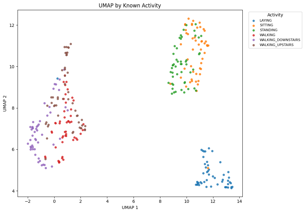
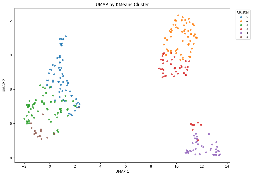
KMeans is trained on PCA features. t-SNE and UMAP are used only to display the activity structure and discovered clusters in two dimensions.
5. Supervised classification with PCA 69#
from sklearn.preprocessing import LabelEncoder

encoder = LabelEncoder()
y_train_encoded = encoder.fit_transform(y_train)
y_test_encoded = encoder.transform(y_test)

encoder.classes_
array(['LAYING', 'SITTING', 'STANDING', 'WALKING', 'WALKING_DOWNSTAIRS',
       'WALKING_UPSTAIRS'], dtype=object)
from joblib import Memory
from sklearn.model_selection import GroupKFold, RandomizedSearchCV
from sklearn.pipeline import Pipeline
from sklearn.metrics import accuracy_score, f1_score, classification_report

cv = GroupKFold(n_splits=3)
cache = Memory("har_pipeline_cache", verbose=0)

results = []
searches = {}
PCA is inside each pipeline, so it is fitted only within the training portion of every cross-validation fold. GroupKFold keeps the recordings of one volunteer together during tuning.
Logistic Regression#
from sklearn.linear_model import LogisticRegression

logistic = Pipeline([
    ("pca", PCA(n_components=69, random_state=42)),
    ("model", LogisticRegression(max_iter=2000))
], memory=cache)

logistic_search = RandomizedSearchCV(
    logistic,
    {"model__C": [0.001, 0.01, 0.1, 1, 10, 100]},
    n_iter=3,
    scoring="f1_macro",
    cv=cv,
    random_state=42,
    n_jobs=1,
    refit=True
)

logistic_search.fit(X_train, y_train_encoded, groups=groups_train)
logistic_pred = logistic_search.predict(X_test)

results.append({
    "Model": "Logistic Regression",
    "CV Macro F1": logistic_search.best_score_,
    "Test Accuracy": accuracy_score(y_test_encoded, logistic_pred),
    "Test Macro F1": f1_score(y_test_encoded, logistic_pred, average="macro")
})

searches["Logistic Regression"] = logistic_search
logistic_search.best_params_
{'model__C': 100}
Random Forest#
from sklearn.ensemble import RandomForestClassifier

forest = Pipeline([
    ("pca", PCA(n_components=69, random_state=42)),
    ("model", RandomForestClassifier(random_state=42, n_jobs=1))
], memory=cache)

forest_search = RandomizedSearchCV(
    forest,
    {
        "model__n_estimators": [50, 80, 120],
        "model__max_depth": [None, 15, 25],
        "model__min_samples_leaf": [1, 2, 4],
        "model__max_features": ["sqrt", "log2"]
    },
    n_iter=2,
    scoring="f1_macro",
    cv=cv,
    random_state=42,
    n_jobs=1,
    refit=True
)

forest_search.fit(X_train, y_train_encoded, groups=groups_train)
forest_pred = forest_search.predict(X_test)

results.append({
    "Model": "Random Forest",
    "CV Macro F1": forest_search.best_score_,
    "Test Accuracy": accuracy_score(y_test_encoded, forest_pred),
    "Test Macro F1": f1_score(y_test_encoded, forest_pred, average="macro")
})

searches["Random Forest"] = forest_search
forest_search.best_params_
{'model__n_estimators': 80,
 'model__min_samples_leaf': 2,
 'model__max_features': 'log2',
 'model__max_depth': 25}
XGBoost#
from xgboost import XGBClassifier

xgb = Pipeline([
    ("pca", PCA(n_components=69, random_state=42)),
    ("model", XGBClassifier(
        objective="multi:softprob",
        num_class=6,
        eval_metric="mlogloss",
        tree_method="hist",
        max_bin=128,
        random_state=42,
        n_jobs=1
    ))
], memory=cache)

xgb_search = RandomizedSearchCV(
    xgb,
    {
        "model__n_estimators": [30, 50, 80],
        "model__max_depth": [3, 5],
        "model__learning_rate": [0.05, 0.10, 0.20],
        "model__subsample": [0.8, 1.0],
        "model__colsample_bytree": [0.8, 1.0]
    },
    n_iter=2,
    scoring="f1_macro",
    cv=cv,
    random_state=42,
    n_jobs=1,
    refit=True
)

xgb_search.fit(X_train, y_train_encoded, groups=groups_train)
xgb_pred = xgb_search.predict(X_test)

results.append({
    "Model": "XGBoost",
    "CV Macro F1": xgb_search.best_score_,
    "Test Accuracy": accuracy_score(y_test_encoded, xgb_pred),
    "Test Macro F1": f1_score(y_test_encoded, xgb_pred, average="macro")
})

searches["XGBoost"] = xgb_search
xgb_search.best_params_
{'model__subsample': 0.8,
 'model__n_estimators': 50,
 'model__max_depth': 3,
 'model__learning_rate': 0.2,
 'model__colsample_bytree': 1.0}
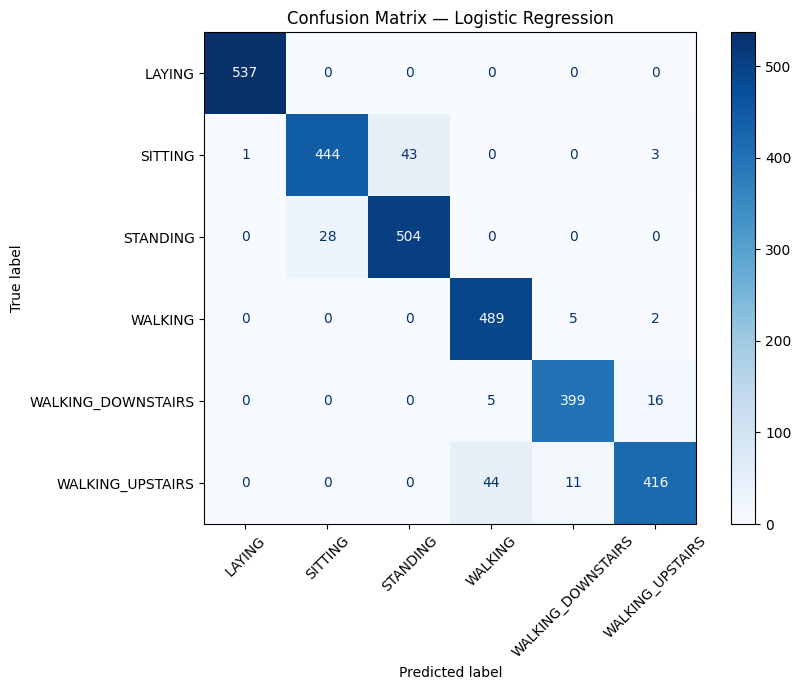
6. Final test-set results#
results_table = (
    pd.DataFrame(results)
    .sort_values("Test Macro F1", ascending=False)
    .reset_index(drop=True)
)

results_table.round(4)
| Model | CV Macro F1 | Test Accuracy | Test Macro F1 | |
|---|---|---|---|---|
| 0 | Logistic Regression | 0.9002 | 0.9464 | 0.9455 |
| 1 | Random Forest | 0.8664 | 0.9084 | 0.9062 |
| 2 | XGBoost | 0.8671 | 0.9036 | 0.9014 |
winner = results_table.loc[0, "Model"]
final_model = searches[winner]
final_prediction = final_model.predict(X_test)

winner
'Logistic Regression'
final_report = classification_report(
    y_test_encoded,
    final_prediction,
    target_names=encoder.classes_,
    output_dict=True
)

pd.DataFrame(final_report).transpose().round(3)
| precision | recall | f1-score | support | |
|---|---|---|---|---|
| LAYING | 0.998 | 1.000 | 0.999 | 537.000 |
| SITTING | 0.941 | 0.904 | 0.922 | 491.000 |
| STANDING | 0.921 | 0.947 | 0.934 | 532.000 |
| WALKING | 0.909 | 0.986 | 0.946 | 496.000 |
| WALKING_DOWNSTAIRS | 0.961 | 0.950 | 0.956 | 420.000 |
| WALKING_UPSTAIRS | 0.952 | 0.883 | 0.916 | 471.000 |
| accuracy | 0.946 | 0.946 | 0.946 | 0.946 |
| macro avg | 0.947 | 0.945 | 0.946 | 2947.000 |
| weighted avg | 0.947 | 0.946 | 0.946 | 2947.000 |
from sklearn.metrics import ConfusionMatrixDisplay

fig, ax = plt.subplots(figsize=(9, 7))

ConfusionMatrixDisplay.from_predictions(
    y_test_encoded,
    final_prediction,
    display_labels=encoder.classes_,
    xticks_rotation=45,
    cmap="Blues",
    ax=ax
)

ax.set_title(f"Confusion Matrix — {winner}")
ax.grid(False)
plt.tight_layout()
plt.show()
Conclusion#
This notebook connects unsupervised and supervised learning in one activity-recognition workflow:
PCA reduces 561 sensor features to compact representations.
KMeans investigates whether activity patterns can be discovered without target labels.
Silhouette, ARI and NMI evaluate the clustering.
t-SNE visualises known activities and discovered groups; a ready-to-run UMAP cell is included for an additional nonlinear visual.
PCA with 69 components is used consistently for classification.
Logistic Regression, Random Forest and XGBoost are tuned with group-aware cross-validation.
The official test volunteers are used only for the final evaluation.