Wholesale Customers Statistical Analysis

Purpose

This notebook answers three simple research questions:

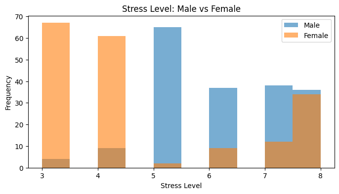
1. Do male and female participants differ in stress level?

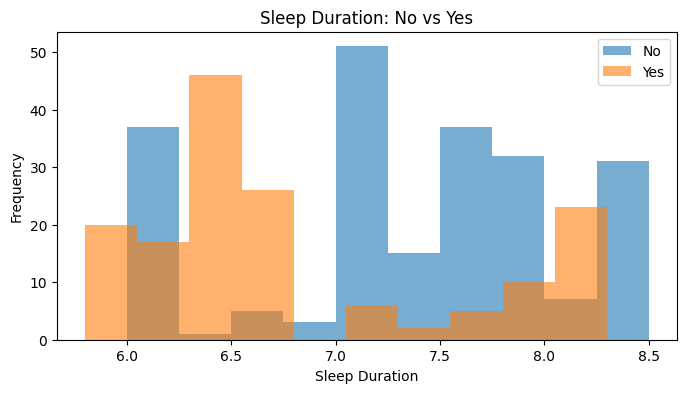
2. Do participants with and without a sleep disorder differ in sleep duration?

3. Do participants with insomnia and sleep apnea differ in physical activity level?

Because each question compares two independent groups, the possible method is either an independent-samples t-test or a non-parametric alternative.
Before testing the questions, we first check whether the compared outcomes behave like normally distributed data.

Statistical decision rule

• Significance level: α = 0.05

• When the group distributions are non-normal or clearly skewed, we use the Mann–Whitney U test

• Since each scenario has only two groups, no post-hoc test is needed

• Levene’s test is not required once we choose Mann–Whitney U, because it is used when deciding how to handle unequal variances in a t-test

import pandas as pd
import numpy as np
import matplotlib.pyplot as plt

from scipy.stats import shapiro, skew, mannwhitneyu

pd.set_option("display.max_columns", None)
pd.set_option("display.float_format", lambda x: f"{x:.4f}")

1. Load and understand the dataset

# The notebook works when the CSV is beside the notebook
# or inside a data folder in a project.

try:
    df = pd.read_csv("sleep.csv")
except FileNotFoundError:
    df = pd.read_csv("../data/sleep.csv")

print("Dataset shape:", df.shape)
display(df.head())

Dataset shape: (374, 13)

	Person ID	Gender	Age	Occupation	Sleep Duration	Quality of Sleep	Physical Activity Level	Stress Level	BMI Category	Blood Pressure	Heart Rate	Daily Steps	Sleep Disorder
0	1	Male	27	Software Engineer	6.1000	6	42	6	Overweight	126/83	77	4200	NaN
1	2	Male	28	Doctor	6.2000	6	60	8	Normal	125/80	75	10000	NaN
2	3	Male	28	Doctor	6.2000	6	60	8	Normal	125/80	75	10000	NaN
3	4	Male	28	Sales Representative	5.9000	4	30	8	Obese	140/90	85	3000	Sleep Apnea
4	5	Male	28	Sales Representative	5.9000	4	30	8	Obese	140/90	85	3000	Sleep Apnea

print("Columns:")
print(df.columns.tolist())

print("\nMissing values:")
display(df.isna().sum().to_frame("Missing Values"))

Columns:
['Person ID', 'Gender', 'Age', 'Occupation', 'Sleep Duration', 'Quality of Sleep', 'Physical Activity Level', 'Stress Level', 'BMI Category', 'Blood Pressure', 'Heart Rate', 'Daily Steps', 'Sleep Disorder']

Missing values:

	Missing Values
Person ID	0
Gender	0
Age	0
Occupation	0
Sleep Duration	0
Quality of Sleep	0
Physical Activity Level	0
Stress Level	0
BMI Category	0
Blood Pressure	0
Heart Rate	0
Daily Steps	0
Sleep Disorder	219

2. Prepare the sleep disorder groups

The original Sleep Disorder column uses missing values for participants who do not have a listed disorder.
We create:

• Sleep Disorder Filled: keeps the three readable categories: None, Insomnia, Sleep Apnea

• Has Sleep Disorder: simplifies the variable into No versus Yes for Scenario 2

df["Sleep Disorder Filled"] = df["Sleep Disorder"].fillna("None")

df["Has Sleep Disorder"] = np.where(
    df["Sleep Disorder"].isna(),
    "No",
    "Yes"
)

display(df["Sleep Disorder Filled"].value_counts().to_frame("Count"))
display(df["Has Sleep Disorder"].value_counts().to_frame("Count"))

	Count
Sleep Disorder Filled
None	219
Sleep Apnea	78
Insomnia	77

	Count
Has Sleep Disorder
No	219
Yes	155

3. Define the three research questions

scenarios = [
    {
        "Question": "Do male and female participants differ in stress level?",
        "Group Column": "Gender",
        "Group 1": "Male",
        "Group 2": "Female",
        "Outcome": "Stress Level"
    },
    {
        "Question": "Do participants with and without sleep disorders differ in sleep duration?",
        "Group Column": "Has Sleep Disorder",
        "Group 1": "No",
        "Group 2": "Yes",
        "Outcome": "Sleep Duration"
    },
    {
        "Question": "Do insomnia and sleep apnea participants differ in physical activity level?",
        "Group Column": "Sleep Disorder Filled",
        "Group 1": "Insomnia",
        "Group 2": "Sleep Apnea",
        "Outcome": "Physical Activity Level"
    }
]

display(pd.DataFrame(scenarios))

	Question	Group Column	Group 1	Group 2	Outcome
0	Do male and female participants differ in stre...	Gender	Male	Female	Stress Level
1	Do participants with and without sleep disorde...	Has Sleep Disorder	No	Yes	Sleep Duration
2	Do insomnia and sleep apnea participants diffe...	Sleep Disorder Filled	Insomnia	Sleep Apnea	Physical Activity Level

4. Check distributions before choosing the test

For each comparison, we examine:

• Skewness: values far from 0 suggest an asymmetric distribution

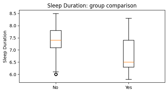
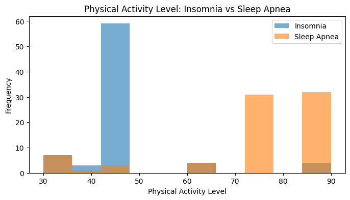
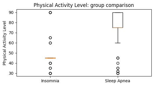
• Shapiro–Wilk test: when p < 0.05, normality is rejected

• Histograms and boxplots: visual evidence of shape and possible outliers

The test choice is based on the evidence below, not selected automatically without checking.

normality_rows = []

for scenario in scenarios:
    for group in [scenario["Group 1"], scenario["Group 2"]]:
        values = df.loc[
            df[scenario["Group Column"]] == group,
            scenario["Outcome"]
        ].dropna()

        shapiro_result = shapiro(values)

        normality_rows.append({
            "Outcome": scenario["Outcome"],
            "Group": group,
            "N": len(values),
            "Median": values.median(),
            "Mean": values.mean(),
            "Skewness": skew(values, bias=False),
            "Shapiro W": shapiro_result.statistic,
            "p-value": shapiro_result.pvalue,
            "Normal at α = 0.05?": "Yes" if shapiro_result.pvalue >= 0.05 else "No"
        })

normality_table = pd.DataFrame(normality_rows)
display(normality_table.round(4))

	Outcome	Group	N	Median	Mean	Skewness	Shapiro W	p-value	Normal at α = 0.05?
0	Stress Level	Male	189	6.0000	6.0794	0.0128	0.8976	0.0000	No
1	Stress Level	Female	185	4.0000	4.6757	0.8544	0.7537	0.0000	No
2	Sleep Duration	No	219	7.4000	7.3584	-0.4315	0.9231	0.0000	No
3	Sleep Duration	Yes	155	6.5000	6.8123	0.7842	0.8325	0.0000	No
4	Physical Activity Level	Insomnia	77	45.0000	46.8182	2.5829	0.5448	0.0000	No
5	Physical Activity Level	Sleep Apnea	78	75.0000	74.7949	-1.3403	0.7578	0.0000	No

for scenario in scenarios:
    group_col = scenario["Group Column"]
    outcome = scenario["Outcome"]
    group_1 = scenario["Group 1"]
    group_2 = scenario["Group 2"]

    x = df.loc[df[group_col] == group_1, outcome].dropna()
    y = df.loc[df[group_col] == group_2, outcome].dropna()

    plt.figure(figsize=(8, 4))
    plt.hist(x, bins=10, alpha=0.6, label=group_1)
    plt.hist(y, bins=10, alpha=0.6, label=group_2)
    plt.title(f"{outcome}: {group_1} vs {group_2}")
    plt.xlabel(outcome)
    plt.ylabel("Frequency")
    plt.legend()
    plt.show()

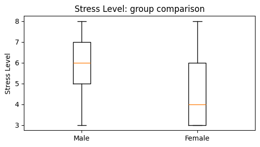
    plt.figure(figsize=(6, 3))
    plt.boxplot([x, y], tick_labels=[group_1, group_2])
    plt.title(f"{outcome}: group comparison")
    plt.ylabel(outcome)
    plt.show()

Method choice

The Shapiro–Wilk results show p < 0.05 for the distributions used in all three comparisons. The plots also help us see the non-normal or uneven shapes of the data.

Therefore, the appropriate method for all three research questions is the Mann–Whitney U test, which compares two independent groups without requiring normal distribution.

Because every comparison contains only two groups:

• Dunn post-hoc testing is not needed

• Levene’s variance test is not needed for the chosen non-parametric test

5. Apply the Mann–Whitney U test

Effect size used: rank-biserial correlation

A p-value tells us whether the group difference is statistically significant.
The effect size tells us how strong the difference is.

Interpretation of the absolute effect size:

• Less than 0.30: small

• 0.30 to less than 0.50: moderate

• 0.50 or above: large

For the direction:

• Positive value: Group 1 generally has higher scores

• Negative value: Group 2 generally has higher scores

def effect_size_label(value):
    absolute_value = abs(value)

    if absolute_value < 0.30:
        return "Small"
    elif absolute_value < 0.50:
        return "Moderate"
    else:
        return "Large"


def run_mann_whitney(data, scenario):
    group_col = scenario["Group Column"]
    group_1 = scenario["Group 1"]
    group_2 = scenario["Group 2"]
    outcome = scenario["Outcome"]

    x = data.loc[data[group_col] == group_1, outcome].dropna()
    y = data.loc[data[group_col] == group_2, outcome].dropna()

    test = mannwhitneyu(
        x,
        y,
        alternative="two-sided",
        method="asymptotic"
    )

    rank_biserial = (2 * test.statistic / (len(x) * len(y))) - 1

    return {
        "Question": scenario["Question"],
        "Outcome": outcome,
        "Group 1": group_1,
        "N1": len(x),
        "Median 1": x.median(),
        "Group 2": group_2,
        "N2": len(y),
        "Median 2": y.median(),
        "U Statistic": test.statistic,
        "p-value": test.pvalue,
        "Significant?": "Yes" if test.pvalue < 0.05 else "No",
        "Rank-Biserial r": rank_biserial,
        "Effect Size": effect_size_label(rank_biserial)
    }

results = []

for scenario in scenarios:
    results.append(run_mann_whitney(df, scenario))

results_table = pd.DataFrame(results)

display(
    results_table[
        [
            "Outcome", "Group 1", "N1", "Median 1",
            "Group 2", "N2", "Median 2",
            "U Statistic", "p-value", "Significant?",
            "Rank-Biserial r", "Effect Size"
        ]
    ].round(4)
)

	Outcome	Group 1	N1	Median 1	Group 2	N2	Median 2	U Statistic	p-value	Significant?	Rank-Biserial r	Effect Size
0	Stress Level	Male	189	6.0000	Female	185	4.0000	25931.0000	0.0000	Yes	0.4833	Moderate
1	Sleep Duration	No	219	7.4000	Yes	155	6.5000	23039.0000	0.0000	Yes	0.3574	Moderate
2	Physical Activity Level	Insomnia	77	45.0000	Sleep Apnea	78	75.0000	910.5000	0.0000	Yes	-0.6968	Large

6. Plain-language interpretation of the results

alpha = 0.05

for number, result in enumerate(results, start=1):
    p_value = result["p-value"]
    r_value = result["Rank-Biserial r"]

    print(f"Scenario {number}: {result['Question']}")
    print(
        f"{result['Group 1']} median = {result['Median 1']}; "
        f"{result['Group 2']} median = {result['Median 2']}."
    )
    print(f"U = {result['U Statistic']:.2f}, p = {p_value:.6f}.")

    if p_value < alpha:
        higher_group = result["Group 1"] if r_value > 0 else result["Group 2"]
        print(
            f"There is a statistically significant difference. "
            f"{higher_group} generally shows higher values on {result['Outcome']}."
        )
        print(
            f"The effect size is {result['Effect Size'].lower()} "
            f"(rank-biserial r = {r_value:.3f})."
        )
    else:
        print("There is no statistically significant difference between the two groups.")

    print()

Scenario 1: Do male and female participants differ in stress level?
Male median = 6.0; Female median = 4.0.
U = 25931.00, p = 0.000000.
There is a statistically significant difference. Male generally shows higher values on Stress Level.
The effect size is moderate (rank-biserial r = 0.483).

Scenario 2: Do participants with and without sleep disorders differ in sleep duration?
No median = 7.4; Yes median = 6.5.
U = 23039.00, p = 0.000000.
There is a statistically significant difference. No generally shows higher values on Sleep Duration.
The effect size is moderate (rank-biserial r = 0.357).

Scenario 3: Do insomnia and sleep apnea participants differ in physical activity level?
Insomnia median = 45.0; Sleep Apnea median = 75.0.
U = 910.50, p = 0.000000.
There is a statistically significant difference. Sleep Apnea generally shows higher values on Physical Activity Level.
The effect size is large (rank-biserial r = -0.697).

7. Final summary

This analysis began by checking the distribution of each outcome inside the groups being compared.
Since the Shapiro–Wilk results rejected normality in all compared distributions and the visual plots supported a non-parametric approach, Mann–Whitney U was applied in all three scenarios.

The notebook reports:

• Group sizes and medians

• Normality evidence before testing

• Mann–Whitney U statistics and p-values

• Rank-biserial effect sizes

• Readable conclusions for each research question

No post-hoc testing is required because none of the analyses compares more than two groups.