IBM HR Employee Attrition: A Statistical Analysis

Project goal

This notebook studies four meaningful questions in the employee dataset. Rather than applying the same test repeatedly, each question uses a method that fits the type of variables involved.

Scenario	Research question	Method
1	Do employees who leave have shorter company tenure than employees who stay?	Mann–Whitney U + rank-biserial effect size
2	Is overtime work associated with employee attrition?	Chi-square + Cramér’s V
3	Is total working experience related to monthly income?	Spearman correlation
4	Does monthly income differ across job roles?	Kruskal–Wallis + Dunn post-hoc

Significance level

Throughout the notebook, the significance level is:

alpha = 0.05

A statistically significant relationship does not prove that one factor causes another. This dataset supports association-based conclusions.

import pandas as pd
import numpy as np
import matplotlib.pyplot as plt

from itertools import combinations
from scipy.stats import (
    shapiro,
    mannwhitneyu,
    chi2_contingency,
    spearmanr,
    kruskal,
    rankdata,
    norm
)

pd.set_option("display.max_columns", None)
pd.set_option("display.float_format", lambda number: f"{number:,.4f}")

alpha = 0.05

1. Load and inspect the dataset

df = pd.read_csv("../data/IBM_HR_Employee_Attrition.csv")

print("Dataset shape:", df.shape)
display(df.head())

Dataset shape: (1470, 35)

	Age	Attrition	BusinessTravel	DailyRate	Department	DistanceFromHome	Education	EducationField	EmployeeCount	EmployeeNumber	EnvironmentSatisfaction	Gender	HourlyRate	JobInvolvement	JobLevel	JobRole	JobSatisfaction	MaritalStatus	MonthlyIncome	MonthlyRate	NumCompaniesWorked	Over18	OverTime	PercentSalaryHike	PerformanceRating	RelationshipSatisfaction	StandardHours	StockOptionLevel	TotalWorkingYears	TrainingTimesLastYear	WorkLifeBalance	YearsAtCompany	YearsInCurrentRole	YearsSinceLastPromotion	YearsWithCurrManager
0	41	Yes	Travel_Rarely	1102	Sales	1	2	Life Sciences	1	1	2	Female	94	3	2	Sales Executive	4	Single	5993	19479	8	Y	Yes	11	3	1	80	0	8	0	1	6	4	0	5
1	49	No	Travel_Frequently	279	Research & Development	8	1	Life Sciences	1	2	3	Male	61	2	2	Research Scientist	2	Married	5130	24907	1	Y	No	23	4	4	80	1	10	3	3	10	7	1	7
2	37	Yes	Travel_Rarely	1373	Research & Development	2	2	Other	1	4	4	Male	92	2	1	Laboratory Technician	3	Single	2090	2396	6	Y	Yes	15	3	2	80	0	7	3	3	0	0	0	0
3	33	No	Travel_Frequently	1392	Research & Development	3	4	Life Sciences	1	5	4	Female	56	3	1	Research Scientist	3	Married	2909	23159	1	Y	Yes	11	3	3	80	0	8	3	3	8	7	3	0
4	27	No	Travel_Rarely	591	Research & Development	2	1	Medical	1	7	1	Male	40	3	1	Laboratory Technician	2	Married	3468	16632	9	Y	No	12	3	4	80	1	6	3	3	2	2	2	2

print("Missing values in the dataset:", df.isna().sum().sum())
print("Duplicate rows:", df.duplicated().sum())

constant_columns = [
    column for column in df.columns
    if df[column].nunique() == 1
]

print("Constant columns:", constant_columns)

df = df.drop(
    columns=[
        "EmployeeNumber",
        "EmployeeCount",
        "Over18",
        "StandardHours"
    ]
)

print("Shape after removing ID and constant columns:", df.shape)

Missing values in the dataset: 0
Duplicate rows: 0
Constant columns: ['EmployeeCount', 'Over18', 'StandardHours']
Shape after removing ID and constant columns: (1470, 31)

Overall attrition summary

Attrition is the central workplace outcome in this project. Before testing possible factors, we first check how many employees left and stayed.

attrition_summary = df["Attrition"].value_counts().rename_axis("Attrition").reset_index(name="Employees")
attrition_summary["Percentage"] = (
    attrition_summary["Employees"] / len(df) * 100
).round(1)

display(attrition_summary)

	Attrition	Employees	Percentage
0	No	1233	83.9000
1	Yes	237	16.1000

2. Scenario 1: Company tenure and attrition

Research question

Do employees who leave have shorter company tenure than employees who stay?

• Grouping variable: Attrition with two independent groups, Yes and No

• Outcome variable: YearsAtCompany

• Since tenure is non-normal inside both attrition groups, the appropriate comparison is the Mann–Whitney U test

• Effect size: rank-biserial correlation

left_tenure = df.loc[df["Attrition"] == "Yes", "YearsAtCompany"]
stayed_tenure = df.loc[df["Attrition"] == "No", "YearsAtCompany"]

tenure_normality = pd.DataFrame({
    "Group": ["Left the company", "Stayed with the company"],
    "N": [len(left_tenure), len(stayed_tenure)],
    "Median Years": [left_tenure.median(), stayed_tenure.median()],
    "Skewness": [left_tenure.skew(), stayed_tenure.skew()],
    "Shapiro p-value": [
        shapiro(left_tenure).pvalue,
        shapiro(stayed_tenure).pvalue
    ]
})

tenure_normality["Normally Distributed?"] = np.where(
    tenure_normality["Shapiro p-value"] >= alpha,
    "Yes",
    "No"
)

display(tenure_normality.round(4))

	Group	N	Median Years	Skewness	Shapiro p-value	Normally Distributed?
0	Left the company	237	3.0000	2.6822	0.0000	No
1	Stayed with the company	1233	6.0000	1.6580	0.0000	No

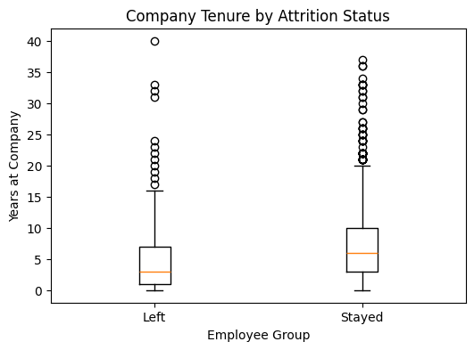
plt.figure(figsize=(6, 4))

plt.boxplot(
    [left_tenure, stayed_tenure],
    tick_labels=["Left", "Stayed"]
)

plt.title("Company Tenure by Attrition Status")
plt.xlabel("Employee Group")
plt.ylabel("Years at Company")
plt.show()

mann_whitney_result = mannwhitneyu(
    left_tenure,
    stayed_tenure,
    alternative="two-sided",
    method="asymptotic"
)

rank_biserial = (
    2 * mann_whitney_result.statistic /
    (len(left_tenure) * len(stayed_tenure))
) - 1

tenure_result = pd.DataFrame({
    "Test": ["Mann–Whitney U"],
    "Median: Left": [left_tenure.median()],
    "Median: Stayed": [stayed_tenure.median()],
    "U Statistic": [mann_whitney_result.statistic],
    "p-value": [mann_whitney_result.pvalue],
    "Rank-Biserial r": [rank_biserial],
    "Significant?": ["Yes" if mann_whitney_result.pvalue < alpha else "No"]
})

display(tenure_result.round(4))

	Test	Median: Left	Median: Stayed	U Statistic	p-value	Rank-Biserial r	Significant?
0	Mann–Whitney U	3.0000	6.0000	102,582.0000	0.0000	-0.2979	Yes

Interpretation

Employees who left the company had a median tenure of 3 years, whereas employees who stayed had a median tenure of 6 years. The difference is statistically significant, and the effect size is close to moderate. This suggests that retention challenges are more visible among employees with shorter organisational tenure.

3. Scenario 2: Overtime and attrition

Research question

Is overtime work associated with employee attrition?

Both variables are categorical:

• OverTime: Yes or No

• Attrition: Yes or No

Therefore, the suitable method is the chi-square test of independence.
Cramér’s V is added to report the strength of the association.

overtime_table = pd.crosstab(df["OverTime"], df["Attrition"])

overtime_rates = (
    pd.crosstab(df["OverTime"], df["Attrition"], normalize="index")
    .mul(100)
    .round(1)
)

display(overtime_table)
display(overtime_rates.rename(columns={"Yes": "Left (%)", "No": "Stayed (%)"}))

Attrition	No	Yes
OverTime
No	944	110
Yes	289	127

Attrition	Stayed (%)	Left (%)
OverTime
No	89.6000	10.4000
Yes	69.5000	30.5000

attrition_rate_by_overtime = overtime_rates["Yes"]

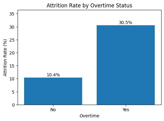
plt.figure(figsize=(6, 4))
plt.bar(attrition_rate_by_overtime.index, attrition_rate_by_overtime.values)

plt.title("Attrition Rate by Overtime Status")
plt.xlabel("Overtime")
plt.ylabel("Attrition Rate (%)")

for position, value in enumerate(attrition_rate_by_overtime.values):
    plt.text(position, value + 0.6, f"{value:.1f}%", ha="center")

plt.ylim(0, attrition_rate_by_overtime.max() + 6)
plt.show()

chi_square_result = chi2_contingency(overtime_table)

chi_square = chi_square_result.statistic
chi_p_value = chi_square_result.pvalue
expected_counts = chi_square_result.expected_freq

n = overtime_table.to_numpy().sum()
cramers_v = np.sqrt(
    chi_square / (n * (min(overtime_table.shape) - 1))
)

risk_ratio = (
    attrition_rate_by_overtime["Yes"] /
    attrition_rate_by_overtime["No"]
)

chi_square_summary = pd.DataFrame({
    "Test": ["Chi-square test"],
    "Chi-square Statistic": [chi_square],
    "p-value": [chi_p_value],
    "Cramer's V": [cramers_v],
    "Minimum Expected Count": [expected_counts.min()],
    "Significant?": ["Yes" if chi_p_value < alpha else "No"]
})

display(chi_square_summary.round(4))
print("Attrition rate risk ratio:", round(risk_ratio, 2))

	Test	Chi-square Statistic	p-value	Cramer's V	Minimum Expected Count	Significant?
0	Chi-square test	87.5643	0.0000	0.2441	67.0694	Yes

Attrition rate risk ratio: 2.93

Interpretation

Employees working overtime had an attrition rate of 30.5%, compared with 10.4% among employees who did not work overtime. The association is statistically significant with a meaningful Cramér’s V effect size. In practical terms, the attrition rate among overtime workers is about 2.93 times the rate among non-overtime workers.

4. Scenario 3: Work experience and monthly income

Research question

Is total working experience related to monthly income?

Both variables are numerical. Since they are not normally distributed, a non-parametric correlation is appropriate:

• Variable 1: TotalWorkingYears

• Variable 2: MonthlyIncome

• Method: Spearman rank correlation

experience = df["TotalWorkingYears"]
income = df["MonthlyIncome"]

correlation_normality = pd.DataFrame({
    "Variable": ["Total Working Years", "Monthly Income"],
    "Skewness": [experience.skew(), income.skew()],
    "Shapiro p-value": [
        shapiro(experience).pvalue,
        shapiro(income).pvalue
    ]
})

correlation_normality["Normally Distributed?"] = np.where(
    correlation_normality["Shapiro p-value"] >= alpha,
    "Yes",
    "No"
)

display(correlation_normality.round(4))

	Variable	Skewness	Shapiro p-value	Normally Distributed?
0	Total Working Years	1.1172	0.0000	No
1	Monthly Income	1.3698	0.0000	No

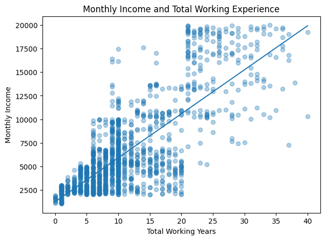
plt.figure(figsize=(7, 5))
plt.scatter(experience, income, alpha=0.35)

trend_values = np.polyfit(experience, income, 1)
trend_line = np.poly1d(trend_values)
ordered_experience = experience.sort_values()

plt.plot(ordered_experience, trend_line(ordered_experience))

plt.title("Monthly Income and Total Working Experience")
plt.xlabel("Total Working Years")
plt.ylabel("Monthly Income")
plt.show()

spearman_result = spearmanr(experience, income)

spearman_summary = pd.DataFrame({
    "Test": ["Spearman Correlation"],
    "Variable 1": ["TotalWorkingYears"],
    "Variable 2": ["MonthlyIncome"],
    "Spearman rho": [spearman_result.statistic],
    "p-value": [spearman_result.pvalue],
    "Significant?": ["Yes" if spearman_result.pvalue < alpha else "No"]
})

display(spearman_summary.round(4))

	Test	Variable 1	Variable 2	Spearman rho	p-value	Significant?
0	Spearman Correlation	TotalWorkingYears	MonthlyIncome	0.7100	0.0000	Yes

Interpretation

There is a strong positive and statistically significant relationship between total working experience and monthly income. Employees with more years of overall work experience generally have higher monthly salaries.

5. Scenario 4: Job role and monthly income

Research question

Does monthly income differ across job roles?

• Grouping variable: JobRole, containing more than two independent groups

• Outcome variable: MonthlyIncome

• Monthly income is skewed, so the suitable test is Kruskal–Wallis

• When the overall test is significant, Dunn post-hoc comparisons with Holm adjustment identify which role pairs differ

role_income_summary = (
    df.groupby("JobRole")["MonthlyIncome"]
    .agg(Employees="count", Median_Income="median", Mean_Income="mean")
    .sort_values("Median_Income")
)

display(role_income_summary.round(2))

	Employees	Median_Income	Mean_Income
JobRole
Sales Representative	83	2,579.0000	2,626.0000
Laboratory Technician	259	2,886.0000	3,237.1700
Research Scientist	292	2,887.5000	3,239.9700
Human Resources	52	3,093.0000	4,235.7500
Sales Executive	326	6,231.0000	6,924.2800
Manufacturing Director	145	6,447.0000	7,295.1400
Healthcare Representative	131	6,811.0000	7,528.7600
Research Director	80	16,510.0000	16,033.5500
Manager	102	17,454.5000	17,181.6800

role_order = role_income_summary.index.tolist()

income_groups = [
    df.loc[df["JobRole"] == role, "MonthlyIncome"]
    for role in role_order
]

plt.figure(figsize=(10, 6))

plt.boxplot(
    income_groups,
    tick_labels=role_order,
    vert=False
)

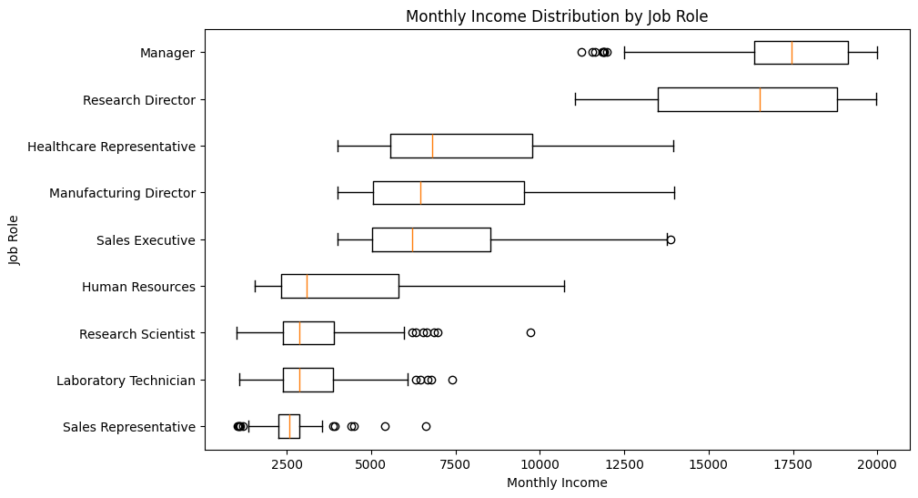
plt.title("Monthly Income Distribution by Job Role")
plt.xlabel("Monthly Income")
plt.ylabel("Job Role")
plt.show()

kruskal_result = kruskal(*income_groups)

epsilon_squared = (
    (kruskal_result.statistic - len(role_order) + 1) /
    (len(df) - len(role_order))
)

kruskal_summary = pd.DataFrame({
    "Test": ["Kruskal–Wallis"],
    "Number of Job Roles": [len(role_order)],
    "H Statistic": [kruskal_result.statistic],
    "p-value": [kruskal_result.pvalue],
    "Epsilon-Squared": [epsilon_squared],
    "Significant?": ["Yes" if kruskal_result.pvalue < alpha else "No"]
})

display(kruskal_summary.round(4))

	Test	Number of Job Roles	H Statistic	p-value	Epsilon-Squared	Significant?
0	Kruskal–Wallis	9	1,073.4101	0.0000	0.7292	Yes

Dunn post-hoc test with Holm correction

Kruskal–Wallis tells us that at least one job role differs in monthly income, but it does not tell us which roles differ. The following small helper function carries out pairwise Dunn comparisons and applies Holm correction so that we do not overstate significance after testing many pairs.

def dunn_posthoc_holm(data, group_col, outcome_col):
    clean_data = data[[group_col, outcome_col]].dropna().copy()
    clean_data["Rank"] = rankdata(clean_data[outcome_col])

    total_n = len(clean_data)
    groups = clean_data[group_col].unique()

    group_counts = clean_data.groupby(group_col).size()
    mean_ranks = clean_data.groupby(group_col)["Rank"].mean()

    ties = clean_data[outcome_col].value_counts()
    tie_sum = ((ties ** 3) - ties).sum()

    rank_variance = (
        total_n * (total_n + 1) / 12
        - tie_sum / (12 * (total_n - 1))
    )

    comparisons = []

    for group_1, group_2 in combinations(groups, 2):
        denominator = np.sqrt(
            rank_variance *
            (1 / group_counts[group_1] + 1 / group_counts[group_2])
        )

        z_value = (
            mean_ranks[group_1] - mean_ranks[group_2]
        ) / denominator

        p_value = 2 * norm.sf(abs(z_value))

        comparisons.append({
            "Group 1": group_1,
            "Group 2": group_2,
            "z": z_value,
            "p-value": p_value
        })

    results = pd.DataFrame(comparisons).sort_values("p-value").reset_index(drop=True)

    number_of_tests = len(results)
    adjusted_values = []

    for index, p_value in enumerate(results["p-value"]):
        adjusted_values.append(
            min((number_of_tests - index) * p_value, 1)
        )

    results["Adjusted p-value"] = np.maximum.accumulate(adjusted_values)
    results["Significant after Holm?"] = np.where(
        results["Adjusted p-value"] < alpha,
        "Yes",
        "No"
    )

    return results


dunn_results = dunn_posthoc_holm(
    data=df,
    group_col="JobRole",
    outcome_col="MonthlyIncome"
)

significant_dunn_results = dunn_results[
    dunn_results["Significant after Holm?"] == "Yes"
]

print("Number of significant pairwise differences:", len(significant_dunn_results))
display(significant_dunn_results.round(4))

Number of significant pairwise differences: 27

	Group 1	Group 2	z	p-value	Adjusted p-value	Significant after Holm?
0	Research Scientist	Manager	-20.5471	0.0000	0.0000	Yes
1	Laboratory Technician	Manager	-20.2427	0.0000	0.0000	Yes
2	Research Scientist	Research Director	-18.2765	0.0000	0.0000	Yes
3	Laboratory Technician	Research Director	-18.0552	0.0000	0.0000	Yes
4	Manager	Sales Representative	17.9813	0.0000	0.0000	Yes
5	Sales Representative	Research Director	-16.6022	0.0000	0.0000	Yes
6	Sales Executive	Research Scientist	16.1414	0.0000	0.0000	Yes
7	Sales Executive	Laboratory Technician	15.6617	0.0000	0.0000	Yes
8	Research Scientist	Healthcare Representative	-13.6251	0.0000	0.0000	Yes
9	Laboratory Technician	Healthcare Representative	-13.3926	0.0000	0.0000	Yes
10	Research Scientist	Manufacturing Director	-13.3204	0.0000	0.0000	Yes
11	Laboratory Technician	Manufacturing Director	-13.0771	0.0000	0.0000	Yes
12	Sales Executive	Sales Representative	12.9765	0.0000	0.0000	Yes
13	Healthcare Representative	Sales Representative	12.3145	0.0000	0.0000	Yes
14	Manager	Human Resources	12.0272	0.0000	0.0000	Yes
15	Manufacturing Director	Sales Representative	11.9740	0.0000	0.0000	Yes
16	Research Director	Human Resources	11.1856	0.0000	0.0000	Yes
17	Sales Executive	Manager	-9.3666	0.0000	0.0000	Yes
18	Sales Executive	Research Director	-8.0612	0.0000	0.0000	Yes
19	Manufacturing Director	Manager	-7.8153	0.0000	0.0000	Yes
20	Healthcare Representative	Manager	-7.0461	0.0000	0.0000	Yes
21	Manufacturing Director	Research Director	-6.8435	0.0000	0.0000	Yes
22	Healthcare Representative	Human Resources	6.8268	0.0000	0.0000	Yes
23	Sales Executive	Human Resources	6.6078	0.0000	0.0000	Yes
24	Manufacturing Director	Human Resources	6.4304	0.0000	0.0000	Yes
25	Healthcare Representative	Research Director	-6.1566	0.0000	0.0000	Yes
26	Sales Representative	Human Resources	-3.4417	0.0006	0.0058	Yes

Interpretation

Monthly income differs significantly across job roles. The median-income table makes the pattern clear: lower-paid roles include Sales Representative, Laboratory Technician and Research Scientist, while Manager and Research Director have the highest median monthly income. Dunn’s post-hoc results show the specific pairs that remain significantly different after correcting for multiple comparisons.

6. Final findings summary

final_summary = pd.DataFrame({
    "Business Question": [
        "Does company tenure differ by attrition?",
        "Is overtime associated with attrition?",
        "Is work experience related to income?",
        "Does income differ across job roles?"
    ],
    "Method": [
        "Mann–Whitney U",
        "Chi-square",
        "Spearman correlation",
        "Kruskal–Wallis + Dunn"
    ],
    "Main Statistical Result": [
        f"U = {mann_whitney_result.statistic:.0f}, p < 0.001, r = {rank_biserial:.3f}",
        f"χ² = {chi_square:.2f}, p < 0.001, V = {cramers_v:.3f}",
        f"ρ = {spearman_result.statistic:.3f}, p < 0.001",
        f"H = {kruskal_result.statistic:.2f}, p < 0.001, ε² = {epsilon_squared:.3f}"
    ],
    "Meaning": [
        "Employees who left had shorter median tenure: 3 vs 6 years.",
        "Overtime employees had 30.5% attrition compared with 10.4% without overtime.",
        "Greater overall experience is strongly related to higher monthly income.",
        "Monthly income differs substantially across job roles."
    ]
})

display(final_summary)

	Business Question	Method	Main Statistical Result	Meaning
0	Does company tenure differ by attrition?	Mann–Whitney U	U = 102582, p < 0.001, r = -0.298	Employees who left had shorter median tenure: ...
1	Is overtime associated with attrition?	Chi-square	χ² = 87.56, p < 0.001, V = 0.244	Overtime employees had 30.5% attrition compare...
2	Is work experience related to income?	Spearman correlation	ρ = 0.710, p < 0.001	Greater overall experience is strongly related...
3	Does income differ across job roles?	Kruskal–Wallis + Dunn	H = 1073.41, p < 0.001, ε² = 0.729	Monthly income differs substantially across jo...

Conclusion

This analysis identifies four meaningful patterns in the employee data:

1. Employees who left tended to have shorter company tenure than those who stayed.

2. Overtime was strongly associated with attrition, with overtime employees leaving at nearly three times the rate of non-overtime employees.

3. Total working experience was strongly positively related to monthly income.

4. Monthly income varied substantially across job roles.

The findings should be treated as associations rather than proof of cause. However, they point toward practical areas for further HR investigation, particularly early-tenure retention and overtime workload.